Introducing ci-proto, our frontier model that says goodbye to context windows and hello to accuracy

State-of-the-art forecasting at your fingertips.

• 2M+ context window. Process 64× the history of any other time-series foundation model.
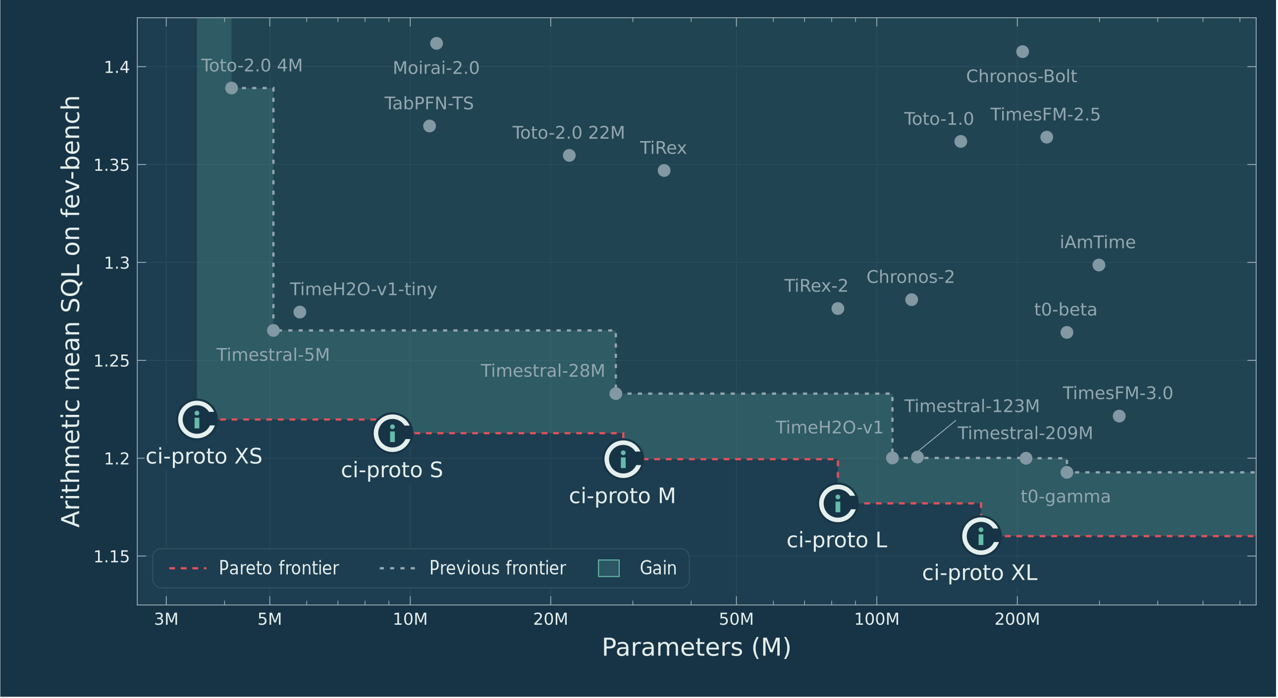
• Frontier accuracy. Leading forecasting performance on fev-bench.
• CPU and GPU support. Run locally through the same Python API.
• Multivariate forecasting. Turn relationships between signals into more accurate forecasts.
• Uncertainty included. Get nine quantiles between 0.1 and 0.9 to plan for a range of outcomes.

Make your first forecast · See the results · Join the waitlist for our next release · Join our Design Partner Program

Make your first forecast

Your first forecast in a few lines. Install with Python 3.10–3.14:

pip install continuousintelligence

Forecast the next day of bicycle rentals from five observed days of hourly demand in Washington, D.C. The example history is included with the package:

import continuousintelligence as ci

# Load the model (uses CUDA when available).
model = ci.load_model("ContinuousIntelligence/ci-proto")

# Load example history as a torch.Tensor shaped [variables, time].
history = ci.load_example()

# Forecast the next 24 hourly time steps.
prediction = model.forecast(history, horizon=24)

# Plot the forecast and its uncertainty bands.
ci.plot_forecast(history, prediction, model.quantiles, output="forecast.png")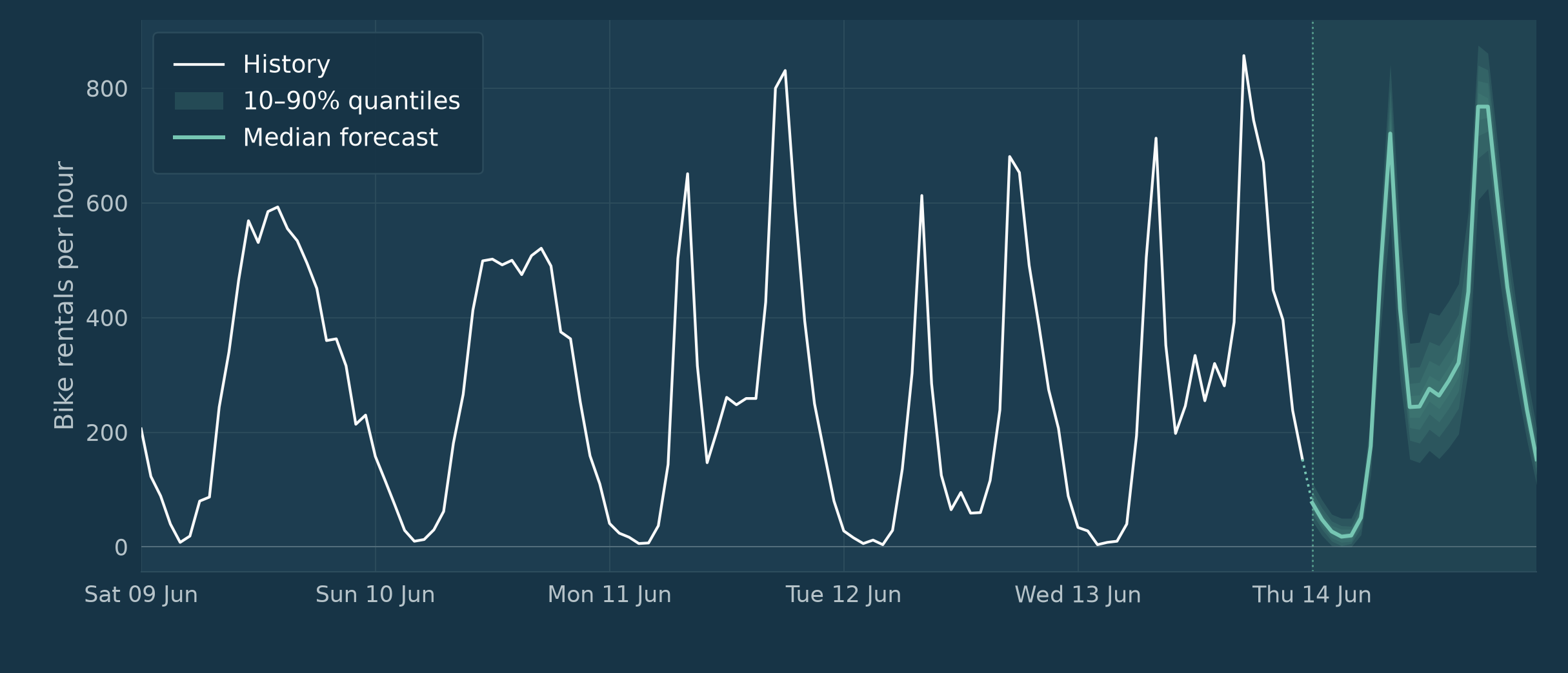

The next 24 hours, with uncertainty included. The shaded region marks the forecast day. The curve shows the model's median forecast, surrounded by nested quantile bands. Replace the example history with your own to get started.

Data: Hadi Fanaee-T (2013), Bike Sharing, UCI, licensed under CC BY 4.0.

Dive deeper. The walkthrough notebook extends this example with calendar covariates, practical uses of the quantiles, and forecasting through missing data.

Frontier performance

The #1 foundation model on fev-bench.

Talk to the team

Tell us what you need to predict. We want to hear about the decisions you're trying to improve, the data you're working with, and where current methods fall short.

Whether you're exploring a new idea or improving an existing system, we'd like to work with you on a solution. Share your use case, your constraints, and what success would look like, and let's discuss how we can help.

Join our Design Partner Program

Beyond ci-proto

Frontier performance is our starting point. ci-proto gives you a first look at our approach to time-series intelligence. Our next release builds on that foundation. Join the waitlist to be the first to hear what's new, see the results, and find out when you can try it.

Join the waitlist

Usage details

Forecast inputs and outputs

Call model.forecast(history, horizon=320) with a two-dimensional PyTorch tensor. Rows are target variables and columns are consecutive time steps. Rows are forecast jointly by default. Supply series_ids to treat them as a cohort of independent univariate series.

In the table below, V is the number of target variables, T is the history length, H is the requested horizon, and Q is the number of quantile levels.

Value	Shape or type	Description
history	[V, T]	Observed target values. Use NaN for missing observations.
horizon	int	Number of future steps to predict. Any positive integer; defaults to 320.
Returned forecast	[V, Q, H]	CPU float32 tensor in the original target units, ordered by quantile level.
model.quantiles	[Q]	CPU tensor containing the probability level for each output quantile.

Input tensors can be real values or NaN. ci-proto returns nine quantiles between 0.1 and 0.9 in increments of 0.1. Histories up to 16,384 observations use the standard checkpoint. Longer histories automatically use the long checkpoint with the full supplied history. The median is the central quantile.

Covariates and categorical inputs

Pass covariates as keyword arguments to model.forecast(..., past_covariates=..., future_covariates=...). Only the variables in history receive forecasts. Align all tensors to the same time axis before calling the model.

Argument	Shape	Requirements
past_covariates	[past_variables, T]	Must have exactly the same history length as history.
future_covariates	[known_variables, T + H]	Must cover both the observed history and the requested forecast horizon.
categorical_past	Tuple of row indices	Selects categorical rows in past_covariates; defaults to ().
categorical_future	Tuple of row indices	Selects categorical rows in future_covariates; defaults to ().

Represent categorical values with numeric category codes. For example, categorical_future=(0, 2) marks its first and third rows as categorical. Boolean covariates can be supplied as numeric inputs without marking them categorical. Use NaN for missing covariate observations.

Timestamps and related series

Pass optional metadata to add calendar features or context from related series.

Argument	Shape or type	Description
timestamps	int64 tensor [T + H] or [V, T + H]	Epoch nanoseconds covering history and horizon. Must increase strictly.
freq	String	Pandas frequency, such as "h", "D" or "W". Required for calendar features.
series_ids	V unique strings	Identifies independent series in input row order.
static_features	Mapping of column names to V values	Optional grouping metadata, such as {"region": ["north", "south"]}. Requires series_ids.

Pass all related series together. Context is shared only between series with the same forecast origin. Covariates can be shared across series or supplied per series as [V, covariates, time].

For uneven histories, left-pad values with NaN and timestamps with torch.iinfo(torch.int64).min.

Loading models and pinning revisions

ci.load_model accepts a Hugging Face repository ID, a local bundle directory, or a checkpoint with a separate calibration file.

model = ci.load_model("ContinuousIntelligence/ci-proto", revision="<commit SHA>")
model = ci.load_model("./local/continuousintelligence")
model = ci.load_model("model.ckpt", "tta.json")

A bundle contains:

local/continuousintelligence/
├── config.json
├── model.ckpt
├── model-long.ckpt
└── tta.json

model.ckpt holds the weights and architecture; tta.json holds preprocessing and calibration settings. model-long.ckpt is the optional long-history checkpoint; it uses the same tta.json and is loaded on the first forecast above the standard context length. config.json describes the model, with its name, parameter count, quantile levels and licence, and is checked against the weights when the model loads. model.info returns it. Hugging Face models always include it; local bundles may omit it.

For reproducibility, pin Hugging Face models with a full commit SHA. revision applies only to Hub loading. Use ./ or a Path object to identify local paths explicitly.

CPU and GPU setup

On Linux, a fresh pip install continuousintelligence installs CUDA-enabled PyTorch. ci.load_model(...) automatically uses an available CUDA GPU, falling back to CPU.

Python versions 3.10–3.14 are supported. On Linux x86-64, installation includes Mamba-3 kernels and the CUDA 13.0.3 toolchain (cuda-toolkit[nvcc,cccl]==13.0.3). Kernels compile on first use and are cached.

device	Behaviour
"auto"	Uses an available CUDA GPU; otherwise CPU. Default.
"cpu"	Uses portable PyTorch inference.
"cuda"	Uses CUDA; raises an error if unavailable.

Fused inference requires CUDA-enabled PyTorch, an Ampere-or-newer NVIDIA GPU, a 580-series-or-newer driver, and a host C++ compiler. Replace CPU-only PyTorch to enable GPU inference.

Inspect model.device and model.backend: "mamba3" means fused CUDA inference; "torch" means the portable backend. Forecast outputs are always CPU tensors.

Reference results use H100 with PyTorch 2.13.0+cu130. Reduced-precision results can vary across runtimes.

Other data and plotting options

ci.plot_forecast(history, prediction, quantiles) works with your own data: history has shape [variables, time], predictions [variables, quantiles, horizon], and the quantile levels form a sorted vector including 0.5 for the median. Each variable gets its own panel with the median and available nested quantile bands. The function returns a Matplotlib figure; output saves it to a file. Pass timestamps covering history plus horizon for a date axis, and ylabel to label the values.

examples/forecast.py forecasts the bundled bicycle-rental history and saves a plot with its dates and units.

Run from the repository root:

pip install .
python examples/forecast.py --model ContinuousIntelligence/ci-proto

The plot is saved to outputs/forecast.png.

To forecast another source, pass --data with a CSV file and name its columns with --time-column and --value-column. If the file has a split column, rows marked history are observed and the following rows marked forecast set the horizon. Otherwise every row is history; pass --horizon, and future timestamps continue the inferred frequency. --ylabel sets the axis label.

python examples/forecast.py --model ContinuousIntelligence/ci-proto \
  --data load.csv --time-column date --value-column load_mw --horizon 48

Use --output for the figure path and --device to select CPU or CUDA. Pin a Hub revision with --revision. Run with --help for all options.

Preprocessing and calibration

Use the checkpoint’s tta.json. Preprocessing, test-time augmentation (TTA), and calibration run automatically without changing model weights.

Setting	Behaviour
postprocess	Enables differencing, band calibration, quantile sorting, and sign-flip averaging.
tta_diff, tta_running_totals	Control trend and running-total differencing.
tta_sign_flip	Averages forecasts of the original and negated inputs.
target_encode_categoricals	Encodes categories using observed target statistics.
clip_nonnegative	Keeps forecasts nonnegative when the observed history is nonnegative.
integer_round	Rounds forecasts when the observed history contains only integers.
calendar_covariates	Adds calendar features when timestamps and frequency are supplied.
bfloat16	Enables reduced-precision inference; false uses float32.

Edit a local tta.json to change these flags. Encoding, clipping, rounding, calendar features, and precision work independently of postprocess.

Keep the supplied numerical constants when reproducing ci-proto results. All configuration fields are required; missing or unknown fields are rejected.

Development

Package structure

Model implementations live in subpackages such as continuousintelligence.ci_proto. The public continuousintelligence.load_model entry point, local/Hub file handling and vendored kernels stay at the package level.

Local setup and tests

Development requires Python 3.10–3.14 and uv 0.11.30 or later. The repository's .python-version selects Python 3.13; CI runs on Python 3.10, 3.13 and 3.14.

From the root of a source checkout, install the locked development dependencies:

uv sync --locked

Development uses the same PyTorch distribution as a normal package install. On Linux this includes CUDA support; the model automatically selects GPU or CPU at runtime.

Run linting, formatting checks, and the default test suite:

uv run --locked ruff check .
uv run --locked ruff format --check .
uv run --locked pytest

The default tests use small synthetic checkpoints and mock Hub downloads, so ci-proto weights are not required. They cover model loading, forecasting, covariates, calibration, and device selection. CUDA tests are skipped when CUDA is unavailable.

To run the additional tests against local ci-proto weights, set both paths:

CONTINUOUSINTELLIGENCE_CHECKPOINT=./local/continuousintelligence/model.ckpt \
CONTINUOUSINTELLIGENCE_TTA_CONFIG=./local/continuousintelligence/tta.json \
uv run --locked pytest -q

Those tests load the supplied checkpoint on CPU and CUDA when available, and check multivariate forecasts at the default horizon, finite outputs, and quantile ordering. Without both environment variables, they are skipped.

Model weights, local calibration files, and generated plots are ignored by Git.

Contributing

Bug reports, feature suggestions, documentation improvements, and code contributions are welcome.

• Report a bug. Include a minimal reproducer, expected and actual behaviour, relevant error output, and your package, Python, and PyTorch versions. Specify whether you are running on CPU or CUDA.
• Suggest a change. Describe the use case, the limitation you have encountered, and the behaviour you would like to see.
• Open a pull request. Explain the problem, the change, and how you verified it. Include a regression test for bug fixes and update the documentation when public behaviour changes.

Small, reproducible examples help us investigate issues and review changes. Keep pull requests focused, and run the checks above before submitting.

Licence

The code and model weights are released under the ci-proto Code and Model Licence. Third-party components retain their upstream licences; see NOTICE for attribution and the Apache 2.0 licence text. The bundled example data is licensed under CC BY 4.0; see its notice.